Microsoft has a tool for running simulated phishing attacks on your Office 365 users. Assuming you are licensed for this tool and wish to do some evaluation of how well your users are doing over time, the built-in MS tools are lacking. Sure you can evaluate a singular test, but really as you train your users and test them you want to be able to see improvement over time as the goal is really to have no one ever click on a phishing link. So how do we gather the results easily?

The first part of that task is to retrieve the data from Microsoft. Microsoft has functionality built into their MS graph API that allows for the retrieval of the data in the scope of 'attacksimulation.read.all'

So start your PowerShell script by connecting to MSgraph:

connect-mggraph -scopes "AttackSimulation.Read.All"

Next, we want to get the list of simulations that have been run, and if needed, we can select only relevant ones. When I run a test simulation, meaning I send it to myself to see what it might look like, I use the word 'test' in the name of the simulation, so I can filter on that. Additionally, Microsoft changed the data that is available in November of 2022, so pulling data before that time isn't as worthwhile (to me) so I've filtered that as well.

$simulations=Get-MgSecurityAttackSimulation -all

#select only the simulations we want
$simulations=$simulations |where {-not($_.displayname -match 'Test') -and $_.createddatetime -gt '11/1/2022'}

Now we can loop through those simulations to get the info we want.

$value=[System.Collections.ArrayList]::new()
foreach($sim in $simulations){
    $url="https://graph.microsoft.com/v1.0/security/attackSimulation/simulations/"+$sim.id +"/report/simulationusers"
    $result=invoke-mggraphrequest -method get $url
    $temp=$result.value
    #if the $result has a '@odata.nextLink' then get results from that link as well
    Do{
        $result=invoke-mggraphrequest -method get $result.'@odata.nextLink'
        $temp+=$result.value
    }While ($null -ne $result.'@odata.nextLink')
    #$value.simulationuser.email|measure
    $temp|add-member -MemberType NoteProperty -name LaunchDateTime -Value $sim.LaunchDateTime
    $value+=$temp
}

From here you can store those values in a local SQL database or flat file. For demonstration purposes, I'm going to use the PowerShell module 'importexcel'.

First I'm going to modify my object a bit to get the data I'm interested in displaying, and the last line exports it to wherever I set $filepath to:

$report=[System.Collections.ArrayList]::new()
foreach ($obj in $value){
    $reportobj=[pscustomobject]@{
        user=$obj.simulationuser.email
        testDatetime=$obj.LaunchDateTime
        successfullydeliveredemail=$($obj.simulationevents|where {$_.eventname -eq 'successfullydeliveredemail'}).eventdatetime
        messageread=$($obj.simulationevents|where {$_.eventname -eq 'messageread'}).eventdatetime
        messagedeleted=$($obj.simulationevents|where {$_.eventname -eq 'messagedeleted'}).eventdatetime
        messagereported=$obj.reportedphishdatetime
        emaillinkclicked=$($obj.simulationevents|where {$_.eventname -eq 'emaillinkclicked'}).eventdatetime
        credsupplied=$($obj.simulationevents|where {$_.eventname -eq 'credsupplied'}).eventdatetime
        attachmentopened=$($obj.simulationevents|where {$_.eventname -eq 'attachmentopened'}).eventdatetime
        outofoffice=$($obj.simulationevents|where {$_.eventname -eq 'outofoffice'}).eventdatetime
        messageforwarded=$($obj.simulationevents|where {$_.eventname -eq 'messageforwarded'}).eventdatetime
        messagereplied=$($obj.simulationevents|where {$_.eventname -eq 'messagereplied'}).eventdatetime
        failedtodeliveremail=$($obj.simulationevents|where {$_.eventname -eq 'failedtodeliveremail'}).eventdatetime
    }
    $report+=$reportobj
}

$report|export-excel $filepath -WorksheetName 'Ticketreporting' -ClearSheet -AutoSize -TableName 'Table1' -Show

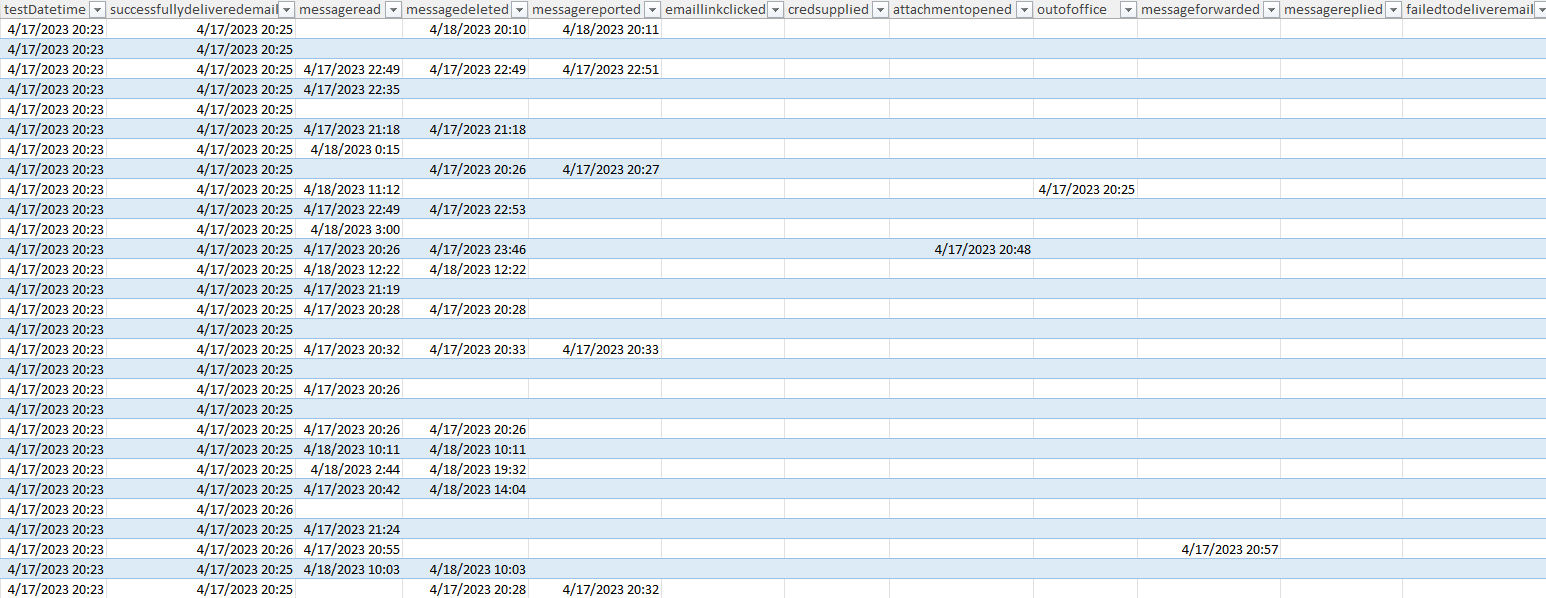
That last line will open Excel and I get a sheet that looks like this (note, the names column has been redacted.)

Great! We have data! Now how do we measure it...? To do this we need to weigh the actions that users are doing. I could make some very convoluted Excel statement that weighs actions, but I want to be able to go back and change weights if I want/need to in the future, so I'm going to make a helper sheet. Things that can happen:

1. mail delivered

2. mail read

3. mail deleted

4. mail reported

5. phishing clicked

6. Supplied credentials

7. attachment opened

8. Out of office

9. Forwarded email

10. Replied to Email

So we want to be able to add up what is in one row to see what a person did, so we can't use the numbers in that list, instead, we need to use powers of 2 so that when we add up everything a person did they can be distinct.

On my helper sheet I setup columns so that they aligned with the exported data:

Back on the data tab, I add a column to the report with the following formula:

=@SUMIF(C2:J2,">0",helper!A$2:J$2)

Now I need to weigh the values. For the sake of brevity, I've excluded the ones for out-of-office, forwarded and replied. I also put this table on my helper tab.

Value	Desc	Weight
0	broken test	0
1	Did not read	2
3	read	-1
5	Deleted without reading	5
7	Read and deleted	4
9	Reported without reading or deleting	15
11	Read and Reported	14
13	Reported and deleted without reading	15
15	read, reported and deleted	14
19	Clicked	-8
23	clicked and deleted	-13
27	Clicked and reported	-5
31	clicked, reported and deleted	-4
51	clicked and supplied creds	-10
55	clicked and supply creds & deleted	-15
59	clicked, supplied creds, reported & deleted	-9
63	clicked and supply creds & reported	-9
67	Attachment opened	-10
71	Attachment opened & deleted	-15
79	Attachment opened & reported	-9

My weighting is based on a +/- 15 point scale and used for example. For your environment, determine your own scale and weigh each action a user could take individually.

Back on the data tab, I add another column for weight with my previously calculated column being N and my weighing table being helper!$A$9:$C$29

The formula in my new column is below but yours could differ if you have more actions weighted (like those forwarded or replied actions):

=@VLOOKUP(N2,helper!$A$9:$C$29,3,FALSE)

I should also note that you can go back to the script that makes the Excel file and insert these additional columns using the ImportExcel module too for future use.

On a new sheet, I made a pivot table/chart that averaged the weight column.

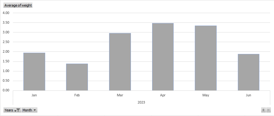
From this, we can see that our training in March-April had an effect, but the positive effects dropped off by June, which at the time of this writing the industry standard is to have a quick 5-10 minute phishing training about every quarter which our data supports.

Now that I have an overall trend, I wanted a little bit more detail. For instance, how many users in my test reported the email without compromise? Pretty easy to count that using Excel, but I wanted to turn it up a notch and separate it by the month that the test occurred in.

On a new sheet, I started by making a row like this:

Test Month

Nov-22

Dec-22

I then made simple calculations to find the month and year in separate cells:

Month	11	12
Year	2022	2022

The formula for 'Month' is: =MONTH(B1) and 'Year' is =YEAR(B1). For future reference, these were made on rows 10 and 11. These formulas can be dragged to the right for however many columns you have.

Starting at row 13 I made these fields:

Months result range start	2	118
Months Result Range End	117	255
Weight range	dataO2:O117	data!O118:O255

Formulas to figure out where your ranges start and end on the 'data' sheet which is where table1 lives:

The first 'Months result range start' cell is set to:

=MATCH(DATE(B$11,B$10,1),DATE(YEAR(Table1[testDatetime]),MONTH(Table1[testDatetime]),1),0)+1

The first 'Months Result Range End' cell is set to:

=MATCH(2,1/(DATE(YEAR(Table1[testDatetime]),MONTH(Table1[testDatetime]),1)=DATE(B$11,B$10,1)))+1

Then the 'Weight Range' fields are a concatenation of strings to figure out what range of cells have the weights we are looking for.

=CONCATENATE("Ticketreporting!O",B$13,":O",B$14)

Looking at different values for the weight and using the 'Indirect' function I was able to put together a table that looked something like this:

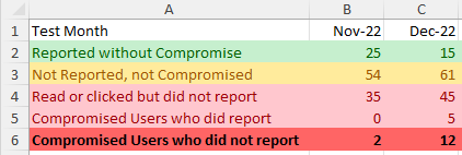
For example, users reported without compromise are found by the following formula =COUNTIF(INDIRECT(B$15),">=10") where B15 is my 'Weight range' that I concatenated in the step before this. As another example, my formula for users that read or clicked but did not report is set to: =COUNTIF(INDIRECT(B$15),"=-1")+COUNTIF(INDIRECT(B$15),"=-8")

If your weights differ from mine, you would need to customize those formulas for your specific weights.

In the end, I now have a PowerShell script and an Excel file that when I run them gives me a quick dashboard view of how the company has done for the monthly phishing simulation that I can track over time, and if needed go review problematic users and assign them additional training sessions.